

This post will help you to enhance your data credibility and learn more about advanced chart configuration.
1- Type Jan in cell A1. You will save your time by using the “Auto Fill” feature. In cell A1
move your mouse to the little handle in the bottom-right corner, the mouse handle will turn into a black cross (see picture below).

2- Click and drag until L1 to use the “Auto Fill” feature.

3- Type the values in figure below.

4- Select Range A1:L2. Go to "Home" tab, "Borders" and "All borders.

5- Go to "Page Layout"' tab, "Sheet Options" and deselect Grid lines View.

6- Go to "Insert" tab, "Charts" group, "Insert Line Chart" and select "Line with Markers".

7- Right click the Vertical axis on the chart and select "Format Axis".

8- Go to "Axis Options", "Bounds" and type Minimum 0 and Maximum 200.

9- Select chart. Go to "Chart Elements", "Gridlines" and check only "Primary major Vertical".

10- Right Click the Horizontal Axis. Go to "Format Axis", "Axis Options", "Tick Marks", "Interval Between Marks" and type 3.

11- Go to "Chart Elements" and Deselect "Axes" or just select axes and press "Delete" key.

12 - Right click the Chart Series (line) and select "Format Data Series". Go to "Fill & Line", select "Markers" and set as Figure below.

13- Border Color will be "Light Gray, Background 2, Darker 75%" and "Width" 3.25 pt.

14- Go to Line change the Color to " Light Gray, Background 2, Darker 75%" and "Width" 3.25 pt.

15- Select the Horizontal Axis and go to "Format Major Gridline", "Line" change color, width to 1.5 pt and "Dash Type" to Dash.

16- Save the five images below by right clicking the image and select "Save image as"


17- Go to "Insert" tab, "Illustrations" group, click in "Picture" and choose the images that you just saved.

18- For the seasons icons. Go to "Format" tab, "Size" group and set "Height" 1.5 cm.
19- The Sunglasses picture will have "Height" 3.5 cm and "Width" 3.48 cm
19- The Sunglasses picture will have "Height" 3.5 cm and "Width" 3.48 cm

20- Select, click and drag the figures to the position as same as figure below.

21- Select Chart. Go to "Format Tab", "Shape Styles Group", "Shape Outline" and select "No Outline".

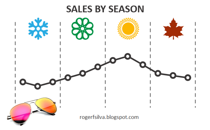
22- At Chart Title, type SALES BY SEASON.

23- Congratulations! You have created a Customized Chart by using advance configuration and figures. If you have any question, try the video in the end of this post.
If you want to learn more about using charts, shapes and pictures to create visual content, try my book "Dynamic Infographic":
If you like the post, please share by clicking on buttons below :)


No comments:
Post a Comment